Evaluating the Impact of Drought Using Remote Sensing Methods
Drought Ravages Lake Mead, Nevada: A Comprehensive Look at the Devastating Impact from 2000 to 2022
-
![]()
Drought Impact on Lake Mead in Nevada (2000-2022)
Lake Mead, located in Nevada, is one of the largest reservoirs in the United States and a critical water source for millions of people in the southwestern region of the country (National Park Service, 2022). However, between 2000 and 2022, significant and continually increasing drought conditions have impacted Lake Mead's water levels and overall health (National Park Service, 2017).
-
![]()
Water Levels and Declining Reserves
The years leading up to 2000 were relatively stable for Lake Mead, with the reservoir operating near full capacity (Carlowicz, 2022). However, drought conditions intensified around 2000, resulting in a prolonged freshwater deficit. As a result, the water levels in Lake Mead started to decline, and this trend continued over the following years.
-
![]()
Hydrological Impact and Environmental Consequences
Lake Mead's water level decline caused a range of environmental consequences. The exposed shoreline and receding water levels disrupted the fragile ecosystems surrounding the reservoir (Lohan, 2022; National Park Service, 2022). Reduced water availability led to habitat loss for various species of fish, birds, and other wildlife that rely on the lake's resources. Additionally, the increased concentration of pollutants in the remaining water due to decreased dilution further deteriorated the water quality.
-
![]()
Economic Effects
The drought's impact on Lake Mead had severe economic consequences for the region. As the water levels declined, it affected agricultural activities, limiting irrigation for farmers and reducing crop yields (Jones, 2023). The declining water supplies also put pressure on the tourism industry, as recreational activities such as boating and fishing became more challenging due to reduced access and navigational hazards (Irfan, 2023).
-
![]()
Water Supply Challenges
The reliability of the water supply for Nevada and neighboring states became increasingly uncertain (Naishadham & Metz, 2022). Numerous water districts and municipalities that rely on Lake Mead as a primary water source were compelled to consider alternative strategies, such as exploring groundwater sources and implementing water conservation measures.


Enhancing Drought Impact Studies: Harnessing Variations in Reflectance for Land and Water Land Cover Types Through Spectral Composites in Remote Sensing Imagery
-
The selected band combination aims to produce a spectral composite that emphasizes the difference between land and water consisting of bands 5, 6, and 4 from Landsat 9. For Landsat 9, Band 5 corresponds to the Near-Infrared (NIR) wavelength ranging from 0.85 - 0.88 μm (Landsat Missions, 2021). Band 6 contains the SWIR 1 wavelength ranging from 1.57 - 1.65 μm. Landsat 9's Band 4 corresponds to the Red wavelength ranging from 0 .64 - 0.67 μm. For this composite, Band 5 was loaded into the Red band, Band 6 was loaded into the Green band, and Band 4 was loaded into the Blue band.
-
The combination of bands 5, 6, and 4 was selected for many reasons. One advantage of this band combination is the stark boundaries created between water and land features due to the exclusion of shorter wavelengths (Center for Biodiversity and Conservation & American Museum of Natural History, 2008; EOS, 2022). The NIR and SWIR 1 bands are highly advantageous for distinguishing the land and water features. In the NIR and SWIR 1 wavelengths, water features absorb highly and reflect minimally compared to the low absorption and high reflectance of land features such as soil, concrete, asphalt, and vegetation (EOS, 2022; Hively et al., 2021; Jensen, 2016; Okin, 2022c; Quinn, 2001). Water's high absorption in these wavelengths results in the dark blue presentation of the feature, with some regions containing slightly varying shades of blue due to a decrease in water depth (EOS, 2022).
Soil is highly reflective in the sensitive NIR and SWIR 1 bands and presents in a range of shades, including white, light green, medium green, deep green, brownish purple, and bright purple, depending on the composition and moisture levels of the soil (Jensen, 2016; Quinn, 2001). Vegetation is highly reflective and minimally absorptive in the NIR and SWIR 1 bands. Vegetation can be seen present near the top of the northern, eastern, and westernmost fingers of Lake Meade on the map on the following page. Vegetation presents shades ranging from light to bright orange depending on the moisture levels within the feature (Okin, 2022a). The red band in this combination aid in distinguishing vegetation and soil from one another due to the wavelength's affinity to be largely absorbed by chlorophyll and reflected by soil and concrete (EOS, 2022; Quinn, 2001).
Histogram Stretches: How They Work and What They Achieve
-
Histogram stretching, sometimes referred to as contrast stretching, “changes the distribution and range of the digital numbers assigned to each pixel in an image" (Sahidan et al., 2008, p. 1). Since the majority of images do not utilize the "total range of the output device," the contrast between features within an image can be weaker than if the image was enhanced to allow for the pixel value range to reach its full potential (Sahidan et al., 2008; Xue, 2022, p. 34). The two camps of contrast enhancement include linear and non-linear mechanisms (Jensen, 2016).
Linear contrast enhancement "linearly expands the original digital values of the remotely sensed data into a new distribution. By expanding the original input values of the image, the total range of sensitivity of the display device can be utilized. Linear contrast enhancement also makes subtle variations within the data more obvious" (Al-amri et al., 2010, p. 27).
The linear contrast enhancement methods used in this analysis are Minimum Maximum,
Percent Clip, and Standard Deviation histogram stretches. “Non-linear contrast enhancement "often involves histogram equalizations through the use of an algorithm" (Al-amri et al., 2010, p. 27). The non-linear contrast enhancement method used in this analysis is the histogram equalization process which occurs as a part of the Dynamic Range Adjustment applied to the image.
-
Dynamic Range Adjustment (DRA) changes the underlying pixel values of an image only within the specific extent of the image being viewed through a program like ArcGIS Pro (Pitcher, 2022; Simularity, n.d.; W, 2011). DRA is an automated contrast enhancement of the image portion being viewed which utilizes an algorithm to calculate the color depth of the viewing area based on "the brightest value in the image" (Simularity, n.d., para. 2). Color depth is then implemented for histogram equalization. Histogram equalization is a form of nonlinear contrast enhancement in which the algorithm analyzes each band in the image and equally distributes the pixels to classes based on the "cumulative frequency histogram" (Al-amri et al., 2010; Jensen, 2016, p. 288). Next, "the image is converted back to RGB using the equalized Brightness value" (Simularity, n.d. para. 2).
Based on the pixel value distribution, histogram equalization can assign identical values to pixels that originally contained distinctive values or the proximity of originally adjacent pixel values (Jensen, 2016). The equalization stretch allows the use of the entire color range as it brings up the underrepresented tail ends of the data values to be equally represented throughout the image (Okin, 2022b). The equalization stretch increases contrast "the most populated range of brightness values of the histogram (or 'peaks')" and "reduces the contrast in very light or dark parts of the image associated with the tails of a normally distributed histogram" (Al-amri et al., 2010, p. 27). The advantage of DRA is seen in the difference between viewing an image entirely with DRA enabled and then zooming into a smaller subset of the image (Pitcher, 2022). In Dr. Pitcher's Technical Demonstration video "Image Histogram Stretching," he views the entire image with DRA enabled, and the contrast between the water features and the land features is lower than when he zooms in to the portion of the river. The DRA recalculates the histogram equalization based on the subset of the viewed image and produces a higher contrast between the river and the land features.
-
The Minimum Maximum Histogram Contrast Stretch and other forms of linear contrast enhancement are "best applied to remotely sensed images with Gaussian or near-Gaussian histograms" (Jensen, 2016, p. 282). The Lansat 9 image of the greater Las Vegas region sans the enabling of DRA or any stretch types has a near-Gaussian histogram (see Appendix Figure 1). It, therefore, is an ideal candidate for the Minimum Maximum Histogram Stretch. While this is "rarely the case" for images that "contain both land and water bodies," the image shown below likely presents with a near-Gaussian histogram due to the relatively few pixels which contain water features in comparison to many pixels which contain land features (Jensen, 2016, p. 283). The water features' presence in the image can be seen in the lowest value region of the histogram, presenting a typical spectra profile response to the bands (see Appendix Figure 2). The Minimum Maximum stretch manipulates and alters pixel values in images using the calculation of Equations 1 (see Appendix) (Jensen, 2016).
The effect of enabling DRA in conjunction with the Maximum Minimum linear stretch can be seen in Figure 3. It is evident that the pixel values were adjusted, or recalculated, by the Minimum Maximum contrast enhancement. Figure 4 (see Appendix) shows the original pixel values for each band in grey behind each new histogram generated by the Minimum Maximum stretch. The image has become brighter as a whole, evidenced by Figure 4 with the shiting of the histogram peak (Okin, 2022a). It is also evident in Figure 4 that the contrast between the bright soil, concrete, and land features and the much lower-valued water features is increased by the distancing of their values.
For ease of viewing and to compensate for the DRA's impact on the zoomed-in image seen in Figure 3, Figure 5 (see Appendix) provides a comparison of the entire images seen in Figure 1 and Figure 3. Appendix Figure 5 shows an increased brightness of pixels in the image with DRA enabled and Minimum Maximum stretch applied (on the right) in comparison to the image without DRA enabled and no stretch applied. The enhanced contrast between the water and land features seen in the right image shows the power of the DRA and Minimum Maximum stretch. Additionally, the enhancements also provided a greater contrast between soil and vegetation.
-
The Percent Clip method of linear contrast enhancement uses the same formula as the Minimum Maximum contrast enhancement but redefines the mink and maxk vaues, effectively "trim[ming] extreme values from both ends of the histogram" based on a percentage (L3 Harris Geospatial, n.d., para. 2; Okin, 2022a). The Percent Clip contrast enhancement reassigns all pixels containing values that previously resided outside of the newly defined minimum and maximum values are given the minimum or maximum value on their respective side of the histogram (ArcGIS Desktop, n.d.). For example, as shown in Figure 6 (see Appendix), the Percent Clip Minimum and Maximum values, auto-defined by the implementation of the Percent Clip stretch in the toolbar, are 0.25. This indicates that ArcGIS Pro removed 0.25% of values residing at the lower and upper portions of the image value range and reassigned those values to the redefined maximum and minimum at the 0.25% cut-off, respectively (ArcGIS Pro, n.d.a).
Figure 7 (see Appendix) shows that the Percent Clip contrast stretch provided a much stronger brightening effect than the Minimum Maximum contrast stretch seen in Figure 4 (see Appendix). The amplitude of the brightening effect is evidenced by the drastic shift in the histogram peak (Okin, 2022a). For ease of viewing, Figure 8 (see Appendix) provides a comparison of the entire images resulting from the Minimum Maximum (left) and Percent Clip (right) contrast stretches. Figure 8 shows the increased contrast provided by the Percent Clip stretch compared to the Minimum Maximum stretch, evidenced by the stark distinction between water and land features and soil types, vegetation, and man- made materials.
For ease of viewing and to compensate for the DRA's impact on the zoomed-in image seen in Figure 6, Figure 9 compares the entire images seen in Figure 1 and Appendix Figure 6. Figure 9 shows the benefits of utilizing a Percent Clip stretch on an image to increase the accentuation of land and water features.
-
The Standard Deviation linear contrast enhancement stretch also utilizes the formula implemented by the Minimum Maximum contrast enhancement. However, the mink and maxk values of this stretch are defined by the "standard deviation value" (ArcGIS Desktop, n.d., para. 7; Jensen, 2016). Similarly to the Percent Clip stretch, any pixel values outside these newly defined minimum and maximum values are reassigned to the new minimum or maximum values, respectively. For example, in Figure 10 (see Appendix), the autogenerated number of standard deviations selected by ArcGIS Pro when selecting the Standard Deviation stretch type on the toolbar was 2.
Therefore, "the values beyond the second standard deviation" are assigned as the new minimum and maximum values, respectively, while anything in between is linearly stretched (ArcGIS Pro, n.d.b, para. 8).
In Figure 11 (see Appendix), it is evident by the drastic shift of the apex to the right that the Standard Deviation contrast stretch created the largest increase of brightness throughout the image compared to the Minimum Maximum and Percent Clip stretch histograms seen in Figures 4 and 7, respectively (see Appendix). The Standard Deviation stretch's slope is "greater than for a simple min-max contrast stretch" (Jensen, 2016, p. 286). For ease of viewing and to compensate for the DRA's impact on the zoomed-in image seen in Figure 10, Figure 12 provides a comparison of the entire images for all stretches conducted. Evaluating the images side-by-side while viewing the full images, it is debatable whether the Percent Clip or Standard Deviation stretches provides the best contrast between land and water features. The Standard Deviation stretch image contains highly contrasting pixels, with many being dark and many being very light. A quick glance at the four images side by side suggests that the Percent Clip is the easiest version to quickly identify the water feature. However, when zooming in on the water feature of the images, the Standard Deviation stretch with DRA enabled clearly provides the crispest and most contrasted differentiation between land and water features.
Spectral Index Selection
𝑁𝐷𝑊𝐼 = 𝐺𝑟𝑒𝑒𝑛−𝑁𝐼𝑅/𝐺𝑟𝑒𝑒𝑛+𝑁𝐼𝑅
M𝑁𝐷𝑊𝐼 = 𝐺𝑟𝑒𝑒𝑛−𝑆𝑊𝐼𝑅/𝐺𝑟𝑒𝑒𝑛+𝑆𝑊𝐼𝑅
The Modified Normalized Difference Water Index (MNDWI) spectral index was selected for this study. This spectral index was selected due to the improvements made to the NDWI for which the equation can be seen on the left. The intentions of the NDWI are as follows:
(1) maximize reflectance of water by using green wavelengths; (2) minimize the low reflectance of NIR by water features; and (3) take advantage of the high reflectance of NIR by vegetation and soil features. As a result, water features have positive values and thus are enhanced, while vegetation and soil usually have zero or negative values and are suppressed (Xu, 2005, p. 3026).
Unfortunately, as Dr. Xu points out:
the application of the NDWI in water regions with a built-up land background does not achieve its goal as expected. The extracted water information in those regions was often mixed with built-up land noise. This means that many built-up land features also have positive values in the NDWI image (Xu, 2005, p. 3026).
Fortunately, Dr. Xu has concocted a simple solution that accounts for the pitfalls of the NDWI with the MNDWI. This was done through the use of the highly sensitive SWIR band rather than the NIR band. The resulting equation is seen to the left.
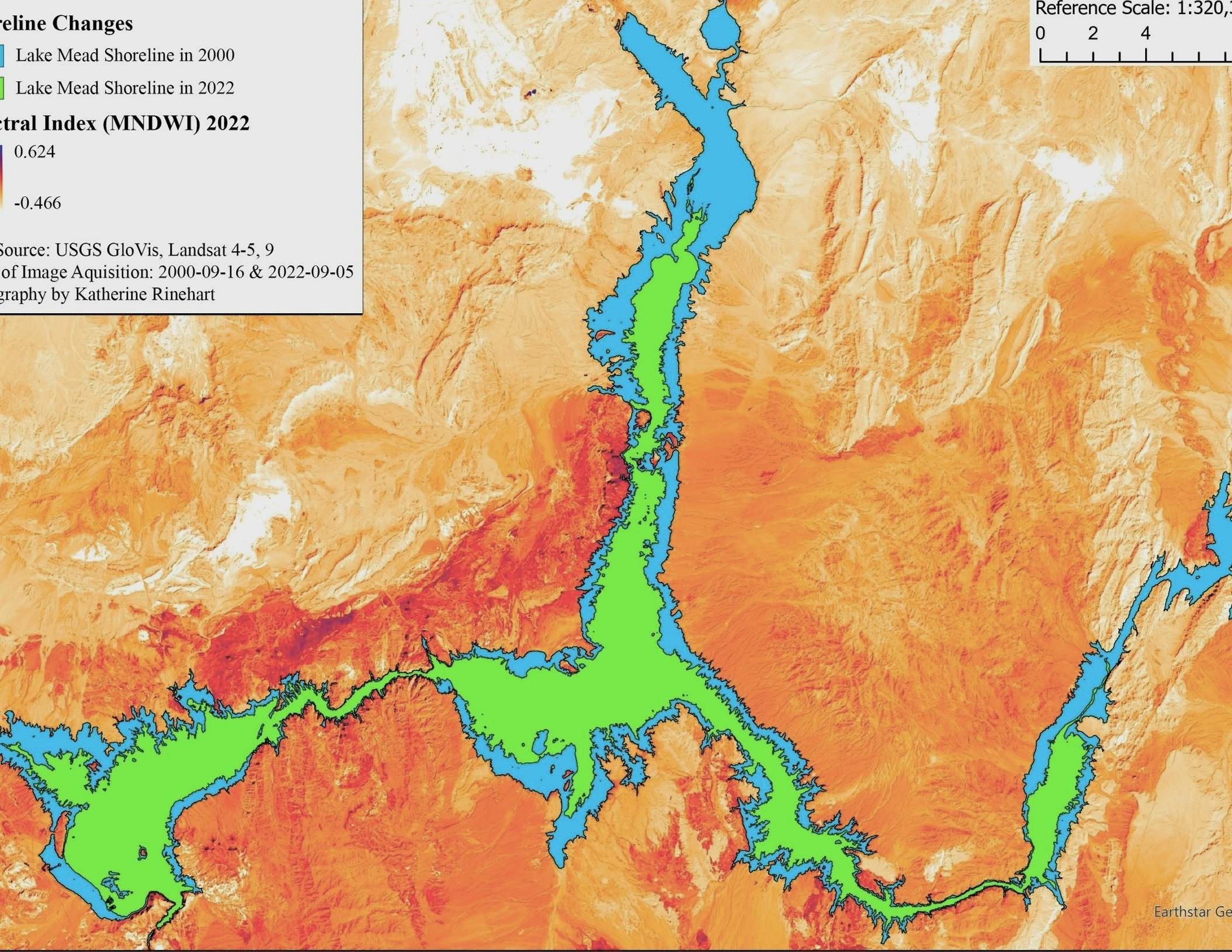
Measuring Lake Mead’s Water Surface Area Changes between 2000 and 2022
ArcGIS Pro was used to map the shoreline for the 2000 and 2022 images of Lake Mead. The vectorized extent of the lake provided measurements for the lake’s water surface area in each year. These values were used to calculate the changes in water surface area between 2000 and 2022. The results of the study are listed below.
Lake Mead Water Surface Area: 2000 and 2022
Lake Mead’s water surface area on September 16, 2000: 552.22 km2 Lake Mead’s water surface area on September 5, 2022: 274.09 km2
Between September 2000 and September 2022, Lake Mead lost 278.13 km2 of water surface area.
Appendix

The Minimum Maximum stretch Equation (Jensen, 2016).

Figure 1. Screen capture of ArcGIS Pro window with Landsat 9 image without DRA enabled or stretch applied and histograms loaded.

Figure 2. A closer view of the histograms provided in Figure 1 to show the water features' presence in histograms.

Figure 3. Screen capture of ArcGIS Pro window with Landsat 9 image with DRA enabled and a Minimum Maximum linear histogram stretch applied and histograms loaded.

Figure 4. A closer view of the histograms provided in Figure 3 to show how the Minimum Maximum linear stretch altered the values of the pixels in the image.

Figure 5. A comparison view of the Landsat 9 image without DRA enabled or stretch applied (left) and the same image with DRA enabled and Minimum Maximum stretch applied (right).

Figure 6. Screen capture of ArcGIS Pro window with Landsat 9 image with DRA enabled and a Percent Clip linear histogram stretch applied and histograms loaded.

Figure 7. A closer view of the histograms provided in Figure 6 to show the water features' presence in histograms and how the Percent Clip linear stretch altered the values of the pixels in the image.

Figure 8. A comparison view of the Landsat 9 image with DRA enabled and Minimum Maximum stretch applied (left) and the same image with DRA enabled and Percent Clip stretch applied (right).

Figure 9. A comparison view of the Landsat 9 image without DRA enabled or stretch applied (left) and the same image with DRA enabled and Percent Clip stretch applied (right).

Figure 10. Screen capture of ArcGIS Pro window with Landsat 9 image with DRA enabled and a Standard Deviation linear histogram stretch applied and histograms loaded.

Figure 11. A closer view of the histograms provided in Figure 10 to show the water features' presence in histograms and how the Standard Deviation linear stretch altered the values of the pixels in the image.

Figure 12. A comparison view of the Landsat 9 image with DRA enabled and Minimum Maximum stretch applied (upper left), the same image with DRA enabled and Percent Clip stretch applied (upper right), the same image with DRA enabled and Standard Deviation stretch applied (bottom left), the same image without DRA enabled and no stretch applied (bottom right).
References
Al-amri, S. S., Kalyankar, N. V., & Khamitkar, S. D. (2010). Contrast Stretching Enhancement in Remote Sensing Image. International Journal of Computer Science Issues (IJCSI), 7(2), 26–29.https://www.proquest.com/docview/89069664/citation/E2A7540FB1DE4E12PQ/1
Carlowicz, M. (2022, July 20). Lake Mead Keeps Dropping [Text.Article]. NASA Earth Observatory; NASA Earth Observatory. https://earthobservatory.nasa.gov/images/150111/lake-mead-keeps-dropping
Center for Biodiversity and Conservation, & American Museum of Natural History. (2008). Landsat Band Information.pdf. Berkeley. http://gif.berkeley.edu/documents/Landsat%20Band%20Information.pdf
ESRI. (n.d.). Imagery appearance—ArcGIS Pro | Documentation. Retrieved October 18, 2022, from https://pro.arcgis.com/en/pro-app/latest/help/data/imagery/raster-display-ribbon.htm
Irfan, U. (2023, April 10). The worst-case scenario for drought on the Colorado River. Vox. https://www.vox.com/the-highlight/23670139/colorado-river-drought-lake-mead-climate-change-water-cuts
Jones, B. (2023, April 10). You—Yes, you—Are going to pay for the century-old mistake that’s draining the Colorado River. Vox. https://www.vox.com/the-highlight/23648116/colorado-river-lake-mead-agriculture-leafy-greens
L3 Harris Geospatial. (n.d.). Stretch Types Background. L3 Harris Geospatail. Retrieved October 18, 2022, from https://www.l3harrisgeospatial.com/docs/backgroundstretchtypes.html
Landsat Missions. (2021). Landsat 9 | U.S. Geological Survey. USGS. https://www.usgs.gov/landsat-missions/landsat-9
Lohan, T. (2022, September 12). Left Out to Dry: Wildlife Threatened by Colorado River Basin Water Crisis • The Revelator. The Revelator. https://therevelator.org/wildlife-colorado-river/
Naishadham, S., & Metz, S. (2022, August 16). Colorado River cuts set to disrupt farming in Western states. PBS NewsHour. https://www.pbs.org/newshour/nation/colorado-river-cuts-set-to-disrupt-farming-in-western-states
National Park Service. (2017, April 4). Drought—Lake Mead National Recreation Area (U.S. National Park Service). National Park Service. https://www.nps.gov/lake/learn/drought.htm
National Park Service. (2022, December 12). Overview of Lake Mead—Lake Mead National Recreation Area (U.S. National Park Service). National Park Service. https://www.nps.gov/lake/learn/nature/overview-of-lake-mead.htm
Okin, G. (2022a). 411.2.1—Contrast stretching & linear stretches (14:20): 22F-GEOG-411- LEC-1 Geospatial Imagery Analysis. BruinLearn. https://bruinlearn.ucla.edu/courses/141360/pages/411-dot-2-1-contrast-stretching-and- linear-stretches-14-20?module_item_id=5376615
Okin, G. (2022b). 411.2.3—Contrast stretching: Other Stretches (9:40): 22F-GEOG-411-LEC-1 Geospatial Imagery Analysis. BruinLearn. https://bruinlearn.ucla.edu/courses/141360/pages/411-dot-2-3-contrast-stretching-other- stretches-9-40?module_item_id=5376617
Pitcher, L. (2022). TD02.02—Image histogram stretching (8:00): 22F-GEOG-411-LEC-1 Geospatial Imagery Analysis. BruinLearn. https://bruinlearn.ucla.edu/courses/141360/pages/td02-dot-02-image-histogram- stretching-8-00?module_item_id=5376625
Sahidan, S. I., Mashor, M. Y., Wahab, A. S. W., Salleh, Z., & Ja’afar, H. (2008). Local and Global Contrast Stretching For Color Contrast Enhancement on Ziehl-Neelsen Tissue Section Slide Images. In N. A. Abu Osman, F. Ibrahim, W. A. B. Wan Abas, H. S. Abdul Rahman, & H.-N. Ting (Eds.), 4th Kuala Lumpur International Conference on Biomedical Engineering 2008 (pp. 583–586). Springer. https://doi.org/10.1007/978-3- 540-69139-6_146
Simularity. (n.d.). Simularity Dynamic Range Adjustment using Histogram Equalization. UP42 Official Website. Retrieved October 18, 2022, from https://up42.com/marketplace/blocks/processing/dra
W, S. (2011). Image Analysis window: What is DRA? ArcGIS Blog. https://www.esri.com/arcgis-blog/products/arcgis-desktop/imagery/image-analysis- window-what-is-dra/