Tmap and Assorted Work

Linear Relationship: GNP and LEXPF - country_demographics.csv

Correlation coefficient between GNP and LEXPF

# set working directory
setwd("C:/Users/data")
country<-read.csv("country_demographics.csv",sep=",",header=T) 
country2<-country[complete.cases(country), ]
countryDF<-as.data.frame(country2)
LEXPF<-countryDF$LEXPF
GNP<-countryDF$GNP
str(LEXPF)

##  num [1:91] 75.5 74.7 77.7 73.8 75.7 72.4 74 75.9 74.8 72.7 ...

str(GNP)

##  int [1:91] 600 2250 2980 2780 1690 1640 2242 1880 1320 2370 ...

cor(GNP,LEXPF)

## [1] 0.6500464

Correlation coefficient, rather than covariance, is the first step in determining the linear relationship between gross national product and the life expectancy of females in the country demographics data set due to impact that variable scales have on covariance values. The correlation coefficient evidences the magnitude of the association between variables on a scale of -1 to 1. The correlation coefficient value is generated using the covariance of the variables and dividing that value by the value of each variables’ standard deviation multiplied by one another. The correlation coefficient for the country_demographics data set is 0.6500464. This value is positive and closer to 1 than it is to 0 suggesting a strong positive relationship. The regression model and t* test-statistic for significance will indicate more about the relationship.

Set hypothesis statement as:
H_0: p = 0
H_A: p != 0

lm<-lm(LEXPF~GNP)
lm

## 
## Call:
## lm(formula = LEXPF ~ GNP)
## 
## Coefficients:
## (Intercept)          GNP  
##    6.09e+01     8.94e-04

summary(lm)

## 
## Call:
## lm(formula = LEXPF ~ GNP)
## 
## Residuals:
##      Min       1Q   Median       3Q      Max 
## -19.8771  -5.8096   0.6023   6.5539  14.1377 
## 
## Coefficients:
##              Estimate Std. Error t value Pr(>|t|)    
## (Intercept) 6.090e+01  1.095e+00   55.60  < 2e-16 ***
## GNP         8.940e-04  1.108e-04    8.07 3.12e-12 ***
## ---
## Signif. codes:  0 '***' 0.001 '**' 0.01 '*' 0.05 '.' 0.1 ' ' 1
## 
## Residual standard error: 8.506 on 89 degrees of freedom
## Multiple R-squared:  0.4226, Adjusted R-squared:  0.4161 
## F-statistic: 65.13 on 1 and 89 DF,  p-value: 3.118e-12

The p-value of 3.118e-12, or 0.000000000003118, is less than the significance level of 0.05. Therefore, the null hypothesis is rejected. Additionally, the coefficients tell us that for every one unit increase in gross national product, there is an 8.940e-04 (or 0.0008940) increase in female life expectancy. Interpretation of these are results using y=mx+b formula is y=0.0008940(x)+60.90. This tells us that with a GNP of $0 the female life expectancy is 60.90 years (variable b in the equation). For each additional unit of GNP, female life expectancy increases by 0.0008940 years (variable m in the equation, also known as the slope).

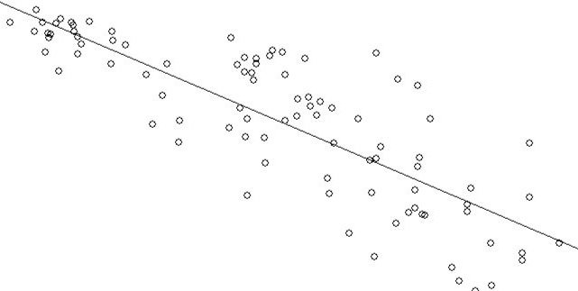
Plotting the Relationship: GNP and LEXPF

plot(GNP,LEXPF)
abline(lm(LEXPF~GNP))

The plot is positively skewed. Let’s look at the plot for this relationship and the accompanying regression line while using log(). Log() will reduce the skew produced by the GNP variable by pulling in outlier values that cause the skew seen in the plot above.

Plotting the Relationship: GNP and LEXPF with log()

logGNP<-log(GNP)
plot(logGNP,LEXPF)
abline(lm(LEXPF~logGNP))

The log() function generated a distribution that is closer to a normal distribution and appears less impacted by skew than the previous plot. From the new plot we can see that the value of b in y=mx+b has decreased significantly, suggestion that the analysis done prior to the log() function was impacted by the skew present in the GNP data.

Recalculating the Correlation Coefficient using the Logged GNP

cor(logGNP,LEXPF)

## [1] 0.8233949

The correlation coefficient value of the relationship, using the logged GNP data, is 0.08233949. This value suggests that the data is more strongly positively correlated than the previous calculation indicated.

Working with Shapefiles

Data Sources: U.S. Census 5-Digit ZIP Code Tabulation Area (ZCTA 5) 2000 - 2019 (Social Explorer). / Colleges and Universities (HIFLD Open Data).

Load Libraries and Shapefiles

library(tmap)
library(tmaptools)
library(raster)

library(sf)

setwd("C:/Users/data")
counties<-st_read("tl_2022_us_county.shp")

## Reading layer `tl_2022_us_county' from data source 
##   `C:\Users\data\tl_2022_us_county.shp' 
##   using driver `ESRI Shapefile'
## Simple feature collection with 3235 features and 17 fields
## Geometry type: MULTIPOLYGON
## Dimension:     XY
## Bounding box:  xmin: -179.2311 ymin: -14.60181 xmax: 179.8597 ymax: 71.43979
## Geodetic CRS:  NAD83

colleges<-st_read("CollegesUniversities.shp")

## Reading layer `CollegesUniversities' from data source 
##   `C:\Users\data\CollegesUniversities.shp' 
##   using driver `ESRI Shapefile'
## Simple feature collection with 6559 features and 43 fields
## Geometry type: POINT
## Dimension:     XY
## Bounding box:  xmin: -19007040 ymin: -1611319 xmax: 19077760 ymax: 11514220
## Projected CRS: WGS 84 / Pseudo-Mercator

Filter Data Sets for California

The CA Counties shapefile mapped by land area in square meters allows the viewer to visualize counties with the largest area. This visualization shows that California counties with the largest area tend to be clustered in the inland desert portion of the state with two large area counties residing in the northern region of the state.

countiesCA <- counties[counties$STATEFP == '06', ]
collegesCA <- colleges[colleges$STATE == 'CA', ]

Map CA Counties using ALAND Variable

tmap_options(check.and.fix = TRUE)
tm_shape(countiesCA)+tm_fill("ALAND", title="Sq. M Area", style = "quantile", n=8, palette = "Blues")+tm_borders()+tm_compass(position = c("LEFT", "BOTTOM"))+tm_layout(main.title = "CA Counties & Area", legend.position = c("RIGHT", "TOP"), title.position = c("center", "top"), inner.margins = .01)+tm_scale_bar(position = c("LEFT", "BOTTOM"))

Map Colleges and CA Counties using ALAND Variable

tm_shape(countiesCA)+tm_fill("ALAND", title="Sq. M Area", style = "quantile", n=8, palette = "Blues")+tm_borders()+tm_compass(position = c("LEFT", "BOTTOM"))+tm_layout(main.title = "CA Counties & Colleges", main.title.size = 1, legend.outside = TRUE, legend.outside.position = "bottom", main.title.position = "LEFT")+tm_scale_bar(position = c("LEFT", "BOTTOM")) + tm_shape(collegesCA) + tm_dots(col = "POPULATION", palette = "Greens", style = "quantile", title = "College Population Size", size = .05)

Point Pattern Analysis

# mean center 
xy<-cbind(collegesCA$LONGITUDE, collegesCA$LATITUDE)
mc<-apply(xy, 2, mean)
mcCA<-st_sfc(st_point(c(mc[1],mc[2])))
mcCA

## Geometry set for 1 feature 
## Geometry type: POINT
## Dimension:     XY
## Bounding box:  xmin: -119.2307 ymin: 35.28371 xmax: -119.2307 ymax: 35.28371
## CRS:           NA

## POINT (-119.2307 35.28371)

tm_shape(countiesCA)+tm_fill("ALAND", title="Sq. M Area", style = "quantile", n=8, palette = "Blues")+tm_borders()+tm_compass(position = c("LEFT", "BOTTOM"))+tm_layout(main.title = "CA Counties & Colleges", main.title.size = 1, legend.outside = TRUE, legend.outside.position = "bottom", main.title.position = "LEFT")+tm_scale_bar(position = c("LEFT", "BOTTOM")) + tm_shape(collegesCA) + tm_dots(col = "POPULATION", palette = "Greens", style = "quantile", title = "College Population Size", size = .05) + tm_shape(mcCA) + tm_dots(col='red',size=.35)

# mean circle 
sd<-sqrt(sum((xy[,1] - mc[1])^2 + (xy[,2] - mc[2])^2) / nrow(xy))
bearing<-1:360 * pi/180
cx<-mc[1]+sd*cos(bearing)
cy<-mc[2]+sd*sin(bearing)
circle<-cbind(cx, cy)
mean_circle<-st_sfc(st_multipoint(circle))

tm_shape(countiesCA)+tm_fill("ALAND", title="Sq. M Area", style = "quantile", n=8, palette = "Blues")+tm_borders()+tm_compass(position = c("LEFT", "BOTTOM"))+tm_layout(main.title = "CA Counties & Colleges", main.title.size = 1, legend.outside = TRUE, legend.outside.position = "bottom", main.title.position = "LEFT")+tm_scale_bar(position = c("LEFT", "BOTTOM")) + tm_shape(collegesCA) + tm_dots(col = "POPULATION", palette = "Greens", style = "quantile", title = "College Population Size", size = .05) + tm_shape(mcCA) + tm_dots(col='red',size=.35) + tm_shape(mean_circle) + tm_dots(col='red',shape=21)

The spatial mean center is calculated by adding all x values together and dividing that value by the total number of observations in the calculation; the same calculation is done with the y values. The result is an average, or mean, coordinate that represents the center of the data. The mean center of the CA Counties and Colleges data is -119.2307, 35.28371 and tells viewers that the average of the coordinate positions resides in Central California, just above the South Coast region.The location suggests that a large number of the California Colleges reside in the Southern coastal region of the state with the next largest density of colleges occurring in the Bay Area region. These high densities result in the mean center residing between the Bay Area and Southern Coast regions of California while remaining closer to the southern portion due to the higher density of colleges in that region.

State Population and Centroids Data Sets

Data Sources: U.S. States and Territories (National Weather Service & NOAA).

Load the Data Sets

setwd("C:/Users/data")
pop<-read.csv("us_state_popln_history.csv",sep=",",header=T) 
centroids<-read.csv("us_state_centroids.csv",sep=",",header=T) 
states<-st_read("tl_2017_us_state.shp")

## Reading layer `tl_2017_us_state' from data source 
##   `C:\Users\data\tl_2017_us_state.shp' 
##   using driver `ESRI Shapefile'
## Simple feature collection with 56 features and 14 fields
## Geometry type: MULTIPOLYGON
## Dimension:     XY
## Bounding box:  xmin: -179.2311 ymin: -14.60181 xmax: 179.8597 ymax: 71.43979
## Geodetic CRS:  NAD83

Filter Data Sets

pop2 <- pop[which(pop$state !="Alaska" & pop$state !="Hawaii"),]
states2 <- states[which(states$NAME !="Alaska" & states$NAME !="Hawaii" & states$NAME !="Commonwealth of the Northern Mariana Islands"  & states$NAME !="American Samoa" & states$NAME !="Puerto Rico" & states$NAME !="United States Virgin Islands" & states$NAME !="Guam"), ]

Dealing with NA Values

In order to deal with the two NA values present in the Oklahoma data for 1870 and 1880, we are going to set NA values to 0 for the calculation of the weighted mean center as missing values will produce an error.

Merging Population Data and the State Shapefile

stpop <- merge(states2, pop2, by.x="NAME", by.y="state")

##      NAME              REGION            DIVISION           STATEFP         
##  Length:49          Length:49          Length:49          Length:49         
##  Class :character   Class :character   Class :character   Class :character  
##  Mode  :character   Mode  :character   Mode  :character   Mode  :character  
##                                                                             
##                                                                             
##                                                                             
##    STATENS             GEOID              STUSPS              LSAD          
##  Length:49          Length:49          Length:49          Length:49         
##  Class :character   Class :character   Class :character   Class :character  
##  Mode  :character   Mode  :character   Mode  :character   Mode  :character  
##                                                                             
##                                                                             
##                                                                             
##     MTFCC             FUNCSTAT             ALAND               AWATER         
##  Length:49          Length:49          Min.   :1.584e+08   Min.   :1.868e+07  
##  Class :character   Class :character   1st Qu.:9.279e+10   1st Qu.:1.540e+09  
##  Mode  :character   Mode  :character   Median :1.389e+11   Median :3.543e+09  
##                                        Mean   :1.562e+11   Mean   :8.744e+09  
##                                        3rd Qu.:2.062e+11   3rd Qu.:8.532e+09  
##                                        Max.   :6.766e+11   Max.   :1.040e+11

##    INTPTLAT           INTPTLON            pop1870           pop1880       
##  Length:49          Length:49          Min.   :      0   Min.   :      0  
##  Class :character   Class :character   1st Qu.:  91874   1st Qu.: 174768  
##  Mode  :character   Mode  :character   Median : 537454   Median : 802525  
##                                        Mean   : 786915   Mean   :1023587  
##                                        3rd Qu.:1184059   3rd Qu.:1542180  
##                                        Max.   :4382759   Max.   :5082871

##     pop1890           pop1900           pop1910           pop1930        
##  Min.   :  47355   Min.   :  42335   Min.   :  81875   Min.   :   91058  
##  1st Qu.: 332422   1st Qu.: 411588   1st Qu.: 577056   1st Qu.:  687497  
##  Median :1118588   Median :1311564   Median :1574449   Median : 1854482  
##  Mean   :1284647   Mean   :1550910   Mean   :1876985   Mean   : 2505613  
##  3rd Qu.:1767518   3rd Qu.:2069042   3rd Qu.:2333860   3rd Qu.: 2939006  
##  Max.   :6003174   Max.   :7268894   Max.   :9113614   Max.   :12588066

##     pop1940            pop1950            pop1960            pop1970        
##  Min.   :  110247   Min.   :  160083   Min.   :  285278   Min.   :  332416  
##  1st Qu.:  663091   1st Qu.:  791896   1st Qu.:  951023   1st Qu.: 1016000  
##  Median : 1901974   Median : 2233351   Median : 2535234   Median : 2824376  
##  Mean   : 2687128   Mean   : 3075456   Mean   : 3642127   Mean   : 4125367  
##  3rd Qu.: 3137587   3rd Qu.: 3444578   3rd Qu.: 4319813   3rd Qu.: 4676501  
##  Max.   :13479142   Max.   :14830192   Max.   :16782304   Max.   :19953134

##     pop1980            pop1990            pop2000            pop2010        
##  Min.   :  469557   Min.   :  453588   Min.   :  493782   Min.   :  563626  
##  1st Qu.: 1302894   1st Qu.: 1515069   1st Qu.: 1808344   1st Qu.: 1852994  
##  Median : 3107576   Median : 3486703   Median : 4041769   Median : 4533372  
##  Mean   : 4595495   Mean   : 5041869   Mean   : 5705784   Mean   : 6258674  
##  3rd Qu.: 5463105   3rd Qu.: 6016425   3rd Qu.: 6349097   3rd Qu.: 6724540  
##  Max.   :23667902   Max.   :29760021   Max.   :33871648   Max.   :37253956

##     pop2020              lon               lat                 geometry 
##  Min.   :  576851   Min.   :-120.56   Min.   :28.63   MULTIPOLYGON :49  
##  1st Qu.: 1961504   1st Qu.:-100.23   1st Qu.:35.86   epsg:4269    : 0  
##  Median : 4657757   Median : -89.20   Median :39.33   +proj=long...: 0  
##  Mean   : 6719604   Mean   : -90.99   Mean   :39.50                     
##  3rd Qu.: 7705281   3rd Qu.: -78.85   3rd Qu.:43.00                     
##  Max.   :39538223   Max.   : -69.24   Max.   :47.45

Weighted Mean Center

x<-stpop2$lon
y<-stpop2$lat
wmx_1870<-weighted.mean(x,stpop2$pop1870)
wmy_1870<-weighted.mean(y,stpop2$pop1870)
wmx_1880<-weighted.mean(x,stpop2$pop1880)
wmy_1880<-weighted.mean(y,stpop2$pop1880)
wmx_1890<-weighted.mean(x,stpop2$pop1890)
wmy_1890<-weighted.mean(y,stpop2$pop1890)
wmx_1900<-weighted.mean(x,stpop2$pop1900)
wmy_1900<-weighted.mean(y,stpop2$pop1900)
wmx_1910<-weighted.mean(x,stpop2$pop1910)
wmy_1910<-weighted.mean(y,stpop2$pop1910)
wmx_1930<-weighted.mean(x,stpop2$pop1930)
wmy_1930<-weighted.mean(y,stpop2$pop1930)
wmx_1940<-weighted.mean(x,stpop2$pop1940)
wmy_1940<-weighted.mean(y,stpop2$pop1940)
wmx_1950<-weighted.mean(x,stpop2$pop1950)
wmy_1950<-weighted.mean(y,stpop2$pop1950)
wmx_1960<-weighted.mean(x,stpop2$pop1960)
wmy_1960<-weighted.mean(y,stpop2$pop1960)
wmx_1970<-weighted.mean(x,stpop2$pop1970)
wmy_1970<-weighted.mean(y,stpop2$pop1970)
wmx_1980<-weighted.mean(x,stpop2$pop1980)
wmy_1980<-weighted.mean(y,stpop2$pop1980)
wmx_1990<-weighted.mean(x,stpop2$pop1990)
wmy_1990<-weighted.mean(y,stpop2$pop1990)
wmx_2000<-weighted.mean(x,stpop2$pop2000)
wmy_2000<-weighted.mean(y,stpop2$pop2000)
wmx_2010<-weighted.mean(x,stpop2$pop2010)
wmy_2010<-weighted.mean(y,stpop2$pop2010)
wmx_2020<-weighted.mean(x,stpop2$pop2020)
wmy_2020<-weighted.mean(y,stpop2$pop2020)

wm_x <- c(wmx_1870, wmx_1880, wmx_1890, wmx_1900, wmx_1910, wmx_1930,wmx_1940, wmx_1950, wmx_1960, wmx_1970,  wmx_1980, wmx_1990, wmx_2000, wmx_2010, wmx_2020)
wm_y<-c(wmx_1870, wmx_1880, wmx_1890, wmx_1900, wmx_1910, wmx_1930,wmx_1940, wmx_1950, wmx_1960, wmx_1970,  wmx_1980, wmx_1990, wmx_2000, wmx_2010, wmx_2020)

wm_xy<-cbind(wm_x,wm_y)
df_wmxy<-data.frame(wm_xy)
uspoints<-st_as_sf(x=df_wmxy,coords=c("wm_x","wm_y"),crs=4326)
# uspoints2<- st_transform(uspoints, crs = "+proj=longlat +datum=NAD83") # tried this but it did not help
years<-c("1870", "1880", "1890", "1900", "1910", "1930", "1940", "1950", "1960", "1970", "1980", "1990", "2000", "2010", "2020")
uspointsYears<-cbind(uspoints,years)

Mapping Weighted Means

tm_shape(stpop2)+tm_polygons()+
tm_shape(uspointsYears)+tm_dots()

stpop2 <- merge(stpop, centroids, by.x="NAME", by.y="state")
stpop2[is.na(stpop2)] = 0
summary(stpop2)