Point Pattern Analysis Using Spatstat
Exploring the Ponderosa Data Set:
Point Pattern, Kernel Density Estimates, Quadrants, Nearest Neighbor Distances, and K Functions
R code is presented in light blue boxes, while the resulting output is provided in light grey boxes.
Point Pattern
data("ponderosa")
X<-ponderosa
plot(X)
The point pattern of the Ponderosa data appears to be random. While some grouping does occur throughout the plot, it does not indicate that the pattern is not consistent with an independent random process at this point in the analysis. However, it is important to remember that it is “often difficult to establish whether first-order effects or second-order effects dominate the spatial point pattern simply by observing a map of events” and further point pattern analysis is warranted.
summary(X)Planar point pattern: 108 points
Average intensity 0.0075 points per square metre
Coordinates are given to 3 decimal places
i.e. rounded to the nearest multiple of 0.001 metres
Window: rectangle = [0, 120] x [0, 120] metres
Window area = 14400 square metres
Unit of length: 1 metreKernel Density
Note that sigma controls smoothing
Kernel density estimations (KDEs) are a local measure of “the density of points over a study region” and is “a test of first-order stationarity” (Baddeley, 2010). The comparison of the KDEs above evidences the two critical parameters of the KDE function. The first parameter is the type of probability density function that is applied to the observations which is determined by the kernel type implemented in the R SpatStat package density function. Each KDE produced has the original point pattern overlaid to aid in the visual assessment of smoothing.
Gaussian Kernel
The Gaussian kernel is commonly used in kernel density estimation (KDE) due to its desirable properties and mathematical characteristics. The Gaussian kernel, also known as the normal distribution or bell curve, is a probability distribution that is symmetric and bell-shaped. It is defined by its mean and standard deviation, which determine the center and spread of the distribution, respectively. When applied in KDE, the Gaussian kernel assigns weights to each data point based on its distance from a given point of interest. The resulting kernel density estimate represents the smoothed probability density function of the underlying data distribution.
# Gaussian - Sigma 7
kd7<-density(X, sigma = 7)
plot(kd7)
plot(X, add=TRUE, cex=0.5)
## Gaussian - Sigma 10
kd10<-density(X, sigma = 10)
plot(kd10)
plot(X, add=TRUE, cex=0.5)# Gaussian - Sigma 45
kd45<-density(X, sigma = 45)
plot(kd45)
plot(X, add=TRUE, cex=0.5)Epanechnikov Kernel
The Epanechnikov kernel grants the sample data points considerably more weight. In contrast with the Gaussian kernel, the projected weights for values surrounding the variable fall to zero more rapidly using the Epanechnikov kernel. The benefits of the Epanechnikov kernel make it a valuable tool in various statistical applications, such as data smoothing and nonparametric regression analysis.
# Epanechnikov - Sigma 7
kdEpan7<-density(X, sigma = 7, kernel=c("epanechnikov"))
plot(kdEpan7)
plot(X, add=TRUE, cex=0.5)
# Epanechnikov - Sigma 10
kdEpan10<-density(X, sigma = 10, kernel=c("epanechnikov"))
plot(kdEpan10)
plot(X, add=TRUE, cex=0.5)# Epanechnikov - Sigma 45
kdEpan45<-density(X, sigma = 45, kernel=c("epanechnikov"))
plot(kdEpan45)
plot(X, add=TRUE, cex=0.5)Disc Kernel
The disc kernel, often referred to as the uniform or rectangular kernel, assigns equal weight to all data points within a specified radius or bandwidth. All data points within this bandwidth are considered equally important in estimating the density at a given point. The choice of bandwidth can affect the smoothness and accuracy of the estimated density function. The disc kernel is particularly useful when the underlying distribution is expected to be relatively smooth and symmetric.
# Disc - Sigma 7
kdDisc7<-density(X, sigma = 7, kernel=c("disc"))
plot(kdDisc7)
plot(X, add=TRUE, cex=0.5)
# Disc - Sigma 10
kdDisc10<-density(X, sigma = 10, kernel=c("disc"))
plot(kdDisc10)
plot(X, add=TRUE, cex=0.5)# Disc - Sigma 45
kdDisc45<-density(X, sigma = 45, kernel=c("disc"))
plot(kdDisc45)
plot(X, add=TRUE, cex=0.5)KDE Results
The kernel types used above are Guassian, Epanechnikov, and Disc. Bivand et al. (2008) state that the most important choice in generating KDEs is the bandwidth, as this metric determines the amount of smoothing that will occur through averaging points per spatial unit. The mechanism in which this works can be seen in the above KDEs; each kernel type is run with bandwidths of 7, 10, and 45 for ease of comparison. In terms of traditional histograms, the bandwidth determines the bin width and how many observations are included in each.
For example, the kd7, kdEpan7, and kdDisc7 KDEs present similarly when the same bandwidth is implemented (Bivand et al., 2008). However, comparing the kdEspan7, kdEspan10, and kdEspan45 to one another reveals drastically different results due to the variation in bandwidth. Looking at kdEspan7, it is evident that the lower bandwidth is producing acceptable amounts of “peaking” while highlighting the regions containing the highest density. On the other hand, looking at the kdEspan45, it is noticeable that the point pattern has been overly smoothed and generalized to the point of only indicating a slight directionality of the points. Of the KDEs generated for each kernel type, a bandwidth value of 7 produced the best results. The results of the KDE show that the Ponderosa density is not uniform and does appear to be clustered in some regions.
Quandrant Count and Test
Xquad<-quadratcount(X, nx=5, ny=5)
plot(X,cex=0.75,pch="+")
plot(Xquad,add=TRUE,cex=1.0)
quadrat.test(X, nx=5, ny=5)Chi-squared test of CSR using quadrat counts
data: X
X2 = 36.444, df = 24, p-value = 0.09934
alternative hypothesis: two.sided
Quadrats: 5 by 5 grid of tilesSignificance level:
α = 0.05
Hypothesis:
HO: the distribution of the points in the Ponderosa data is random and consistent with an independent random process (IRP).
HA: the spatial distribution of the points in the Ponderosa data is not random and inconsistent with an IRP.
Results:
The p-value of 0.09934 is greater than the significance level of 0.05 and, as a result, the null hypothesis is not rejected.
Nearest Neighbor Distances
Xdistmatrix <- pairdist(X)
XnnDist<-nndist(X)
dbarobs<-sum(XnnDist)/length(XnnDist)
dbarobs6.837259dbarexp<-0.5/sqrt(108/14400)
dbarexp5.773503sddbarexp<-.26136/sqrt((108^2)/14400)
sddbarexp0.2904R<-6.837259/5.773503
R1.184248Ztest<-(dbarobs-dbarexp)/sddbarexp
Ztest4.48633Nearest Neighbor analysis is a second-order stationary, distance-based global measure of a data set’s point pattern and is used to determine whether the observed point pattern is clustered, random or dispersed. The R value of 1.184248 is close to 1 indicating that the Ponderosa point pattern is random and consistent with an IRP.
Significance level:
α = 0.05
A two tailed test establishes the z-values as -1.96 and 1.96
Hypothesis:
HO: the distribution of the points in the Ponderosa data is random and consistent with an independent random process (IRP).
HA: the spatial distribution of the points in the Ponderosa data is not random and inconsistent with an IRP.
Results:
The z-score test statistic value of 4.48633 is well outside of the values for the 0.05 significance level and therefore the null hypothesis is rejected with a confidence level of 95%. In fact, even at a confidence level of 99% (significance level of 0.01), the null hypothesis would be rejected. Additionally, the observed value is larger than the expected value indicating a dispersed point pattern.
K Function
kf<-Kest(X, correction='Ripley')
plot(kf)
The K functions plot above shows that the observed values are slightly lower than the expected values at small distances and then slightly higher than the expected values at large distances. Therefore, at large distances there is indication of a potentially clustered pattern and at smaller distances there is indication of a potentially regular or uniform pattern for the Ponderosa data set. Whether these differences are significant or not can be assessed using a K function envelope.
K Function Envelope
kfEnv<-envelope(X,Kest,correction='Ripley')Generating 99 simulations of CSR ...
1, 2, 3, 4, 5, 6, 7, 8, 9, 10, 11, 12, 13, 14, 15, 16, 17, 18, 19, 20, 21, 22, 23, 24, 25, 26, 27, 28, 29,
30, 31, 32, 33, 34, 35, 36, 37, 38, 39, 40, 41, 42, 43, 44, 45, 46, 47, 48, 49, 50, 51, 52, 53, 54, 55, 56, 57, 58,
59, 60, 61, 62, 63, 64, 65, 66, 67, 68, 69, 70, 71, 72, 73, 74, 75, 76, 77, 78, 79, 80, 81, 82, 83, 84, 85, 86, 87,
88, 89, 90, 91, 92, 93, 94, 95, 96, 97, 98, 99.plot(kfEnv)The confidence interval envelope consistently overlaps both the observed and expected values in the K function plot indicating that the observed and expected values are not significantly different and are consistent with an IRP.
Mean Absolute Deviation (MAD) Test
The mean absolute deviation (MAD) is a statistical measure that calculates the average distance between each value in a dataset and the mean of that dataset. It assesses the variability or dispersion of data points around the mean. When applied to k functions, MAD measures the average absolute difference between the values of k different functions and their respective means. MAD provides insights into the consistency or divergence of these functions from their average values. MAD is a useful tool in analyzing data sets with multiple functions, as it concisely quantifies their deviations from their respective means.
mad.test(X,Kest)Generating 99 simulations of CSR ...
1, 2, 3, 4, 5, 6, 7, 8, 9, 10, 11, 12, 13, 14, 15, 16, 17, 18, 19, 20, 21, 22, 23, 24, 25, 26, 27, 28, 29,
30, 31, 32, 33, 34, 35, 36, 37, 38, 39, 40, 41, 42, 43, 44, 45, 46, 47, 48, 49, 50, 51, 52, 53, 54, 55, 56, 57, 58,
59, 60, 61, 62, 63, 64, 65, 66, 67, 68, 69, 70, 71, 72, 73, 74, 75, 76, 77, 78, 79, 80, 81, 82, 83, 84, 85, 86, 87,
88, 89, 90, 91, 92, 93, 94, 95, 96, 97, 98, 99.
Done.
Maximum absolute deviation test of CSR
Monte Carlo test based on 99 simulations
Summary function: K(r)
Reference function: theoretical
Alternative: two.sided
Interval of distance values: [0, 30] metres
Test statistic: Maximum absolute deviation
Deviation = observed minus theoreticaldata: X
mad = 284.95, rank = 4, p-value = 0.04
Significance level:
α = 0.05
Hypothesis:
HO: the distribution of the points in the Ponderosa data is random and consistent with an independent random process (IRP).
HA: the spatial distribution of the points in the Ponderosa data is not random and inconsistent with an IRP.
Results:
The MAD test statistic of 284.95 with a p-value of 0.04, which is smaller than the significance level of 0.05 indicates that the null hypothesis should be rejected and that the data is not random. However, the contradictions between the envelope analysis and the MAD test analysis evidence the issues with a p-value of 0.05 as opposed to a p-value of 0.01.
Exploring the California Air Sites Data Set: Point Pattern, Kernel Density Estimates, Quadrants, Nearest Neighbor Distances, and K Functions
The California Air Sites data set can be downloaded here.
Coercing Point Data
setwd("C:/Users/calairsites")
spatialpoints1<-st_read("airmonitoringstations.shp")
spatialpoints1<-subset(spatialpoints1, ZIPCODE != "xxxxx")      # Remove points located in Mexico to prevent future issues in analysis
spatialpoints2<-as (spatialpoints1, "Spatial")
spatialpoints3 <- as (spatialpoints2, "SpatialPoints")
spatialpoints4 <- as (spatialpoints3, "ppp")

spatialpoly1 <- st_read ("arb_california_airdistricts_aligned_03.shp")
spatialpoly2 <- as (spatialpoly1, "Spatial")
spatialpoly3 <- as (spatialpoly2, "SpatialPolygons")
spatialpoly3 <- as (spatialpoly2, "SpatialPolygons")
spatialpoly4 <- as (spatialpoly3, "owin")

spatialpoints4$window <- spatialpoly4
plot(spatialpoints4)
The point data appears to show clustering around the coastal and central regions near San Fransisco in northern California and most of the southern California coast. As previously stated, it is difficult to determine the nature of the point pattern without further analysis.
First-Order and Second-Order Stationarity
First-Order Stationarity
Kernel Density Estimate
# Gaussian - Sigma 250
CAkd250 <- density(spatialpoints4,sigma=250)
plot(CAkd250)
plot(spatialpoints4, add=TRUE, cex=0.5)
# Gaussian - Sigma 25000
CAkd25000 <- density(spatialpoints4,sigma=25000)
plot(CAkd25000)
plot(spatialpoints4, add=TRUE, cex=0.5)
Point pattern analysis aims to determine whether the pattern is compatible with the independent random process (IRP) or with what we also refer to as complete spatial randomness. If it is consistent with an IRP, the conclusion is that additional investigation is unnecessary because the point pattern is likely to have been created by a random process. Geospatial data scientists are primarily interested in situations when the analysis results do not support the notion that an IRP generated the point pattern. The absence of evidence that the pattern matches an IRP suggests that it was produced by a non-random method and warrants further analysis.
First-order and second-order stationarity is required for a point pattern to have been produced by an independent random process (IRP). The homogeneity of the density of points inside a research region is assumed by first-order stationarity. Events or points must be positioned independently to comply with second-order stationarity, meaning the location of one event is unrelated to the placement of other occurrences.
The Gaussian KDEs above show the impact of different bandwidths for the point data. Due to the high number of points, a large bandwidth value was required to produce appropriate levels of smoothing. The CAkd25000 KDE confirms the interpretation of the original plot of the point data over the study area which stated that clustering was seen near coastal regions.
Quandrant Count and Test
plot(spatialpoints4, add=TRUE, cex=0.5)
quadrat.test(spatialpoints4, nx=6, ny=6)Chi-squared test of CSR using quadrat counts
data: spatialpoints4
X2 = 250.89, df = 23, p-value < 2.2e-16
alternative hypothesis: two.sided
Quadrats: 24 tiles (irregular windows)Significance level:
α = 0.05
Hypothesis:
HO: the distribution of the points in the California Air Sites data is random and consistent with an independent random process (IRP).
HA: the spatial distribution of the points in the California Air Sites data is not random and inconsistent with an IRP.
Results:
The p-value of 2.2e-16 is lower than the significance level of 0.05 and, as a result, the null hypothesis is rejected.
Second-Order Stationarity
Nearest Neighbor Distances
spatialDistMatrix<- pairdist(spatialpoints4)
XnnDistSp<-nndist(spatialpoints4)
dbarobsSp<-sum(XnnDistSp)/length(XnnDistSp)
dbarobsSp14801.17dbarexpSp<-0.5/sqrt(259/4.10598e+11)
dbarexpSp19908.04sddbarexpSp<-.26136/sqrt((259^2)/4.10598e+11)
sddbarexpSp0.2371106Rsp<-14801.17/19908.04
Rsp0.743477ZtestSp<-(dbarobsSp-dbarexpSp)/sddbarexpSp
ZtestSp-7.897826The R value of 0.743477 is close to 1 potentially indicating that the point pattern is random and consistent with an IRP.
Significance level:
α = 0.05
A two tailed test establishes the z-values as -1.96 and 1.96
Hypothesis:
HO: the distribution of the points in the California Air Sites data is random and consistent with an independent random process (IRP).
HA: the spatial distribution of the points in the California Air Sites data is not random and inconsistent with an IRP.
Results:
The z-score test statistic value of -7.897826 is well outside of the range of the 0.05 significance level and therefore the null hypothesis is rejected with a confidence level of 95%. In fact, even at a confidence level of 99% (significance level of 0.01), the null hypothesis would be rejected. Additionally, the observed value is smaller than the expected value indicating a clustered point pattern.
K Function
kfSp<-Kest(spatialpoints4, correction='Ripley')plot(kfSp)The K functions plot above shows that the observed values align with the expected values at very small distances. However, the observed values are significantly higher than the expected values at large distances. Therefore, there is indication of a potentially clustered pattern for the majority of the data except for at very small distances where there is indication of a potentially regular or uniform pattern for the California Air Sites data set. Whether these differences are significant or not can be assessed using a K function envelope.
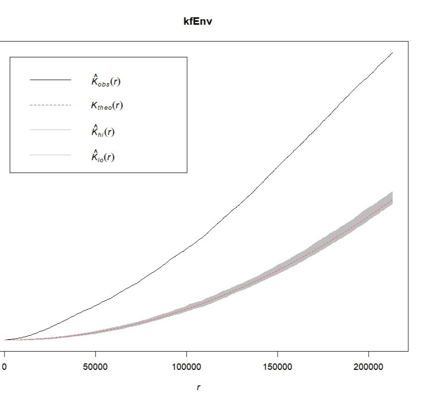
K Function Envelope
kfEnv<-envelope(spatialpoints4,Kest,correction='Ripley')Generating 99 simulations of CSR ...
1, 2, 3, 4, 5, 6, 7, 8, 9, 10, 11, 12, 13, 14, 15, 16, 17, 18, 19, 20, 21, 22, 23, 24, 25, 26, 27, 28, 29,
30, 31, 32, 33, 34, 35, 36, 37, 38, 39, 40, 41, 42, 43, 44, 45, 46, 47, 48, 49, 50, 51, 52, 53, 54, 55, 56, 57, 58,
59, 60, 61, 62, 63, 64, 65, 66, 67, 68, 69, 70, 71, 72, 73, 74, 75, 76, 77, 78, 79, 80, 81, 82, 83, 84, 85, 86, 87,
88, 89, 90, 91, 92, 93, 94, 95, 96, 97, 98, 99.plot(kfEnv)The confidence interval envelope overlaps the expected values in the K function plot but not the observed values, indicating that the observed and expected values are significantly different and that the California Air Sites data is not consistent with an IRP.
MAD Test
mad.test(spatialpoints4,Kest)Generating 99 simulations of CSR ...
1, 2, 3, 4, 5, 6, 7, 8, 9, 10, 11, 12, 13, 14, 15, 16, 17, 18, 19, 20, 21, 22, 23, 24, 25, 26, 27, 28, 29,
30, 31, 32, 33, 34, 35, 36, 37, 38, 39, 40, 41, 42, 43, 44, 45, 46, 47, 48, 49, 50, 51, 52, 53, 54, 55, 56, 57, 58,
59, 60, 61, 62, 63, 64, 65, 66, 67, 68, 69, 70, 71, 72, 73, 74, 75, 76, 77, 78, 79, 80, 81, 82, 83, 84, 85, 86, 87,
88, 89, 90, 91, 92, 93, 94, 95, 96, 97, 98, 99.Done.
Maximum absolute deviation test of CSR
Monte Carlo test based on 99 simulations
Summary function: K(r)
Reference function: theoretical
Alternative: two.sided
Interval of distance values: [0, 213058.741032929]
Test statistic: Maximum absolute deviation
Deviation = observed minus theoretical
data: spatialpoints4
mad = 1.4889e+11, rank = 1, p-value = 0.01Significance level:
α = 0.05
Hypothesis:
HO: the distribution of the points in the California Air Sites data is random and consistent with an independent random process (IRP).
HA: the spatial distribution of the points in the California Air Sites data is not random and inconsistent with an IRP.
Results:
The MAD test statistic of 1.4889e+11 with a p-value of 0.01, which is smaller than the significance level of 0.05 indicates that the null hypothesis should be rejected and that the data is not random. This finding is in agreement with the results of the K function envelope analysis.
References
Baddeley, A. (2010). Analysing spatial point patterns in R.
Bivand, R. S., Pebesma, E. J., & Gómez-Rubio, V. (Eds.). (2008). Spatial Point Pattern Analysis. In Applied Spatial Data Analysis with R (pp. 155–190). Springer. https://doi.org/10.1007/978-0-387-78171-6_7